Beta-Binomial Distribution

Definition (Beta Distribution)

An r.v. $X$ is said to have Beta distribution with parameters $a$ and $b$, if its PDF is

$$f(x) = \frac{1}{\beta(a,b)}x^{a-1}(1-x)^{b-1},0<x<1$$

where $\beta(a,b)$ is constant to make PDF integrate to 1, We write this as $X\sim Beta(a,b)$

By varying the values of $a$ and $b$, we get PDFs with a variety of shapes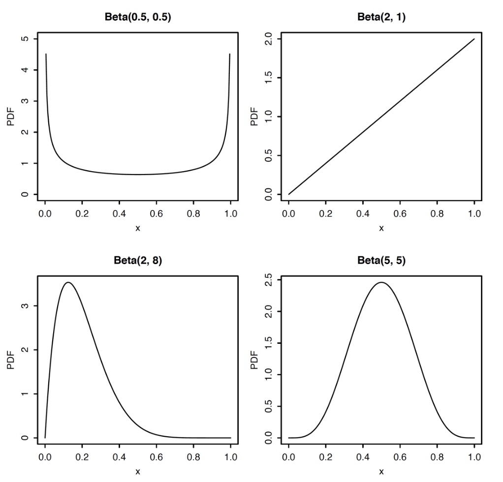

Beta Distribution is the generalization of uniform distribution while $a=b=1$

The Beta is a flexible family of continuous distributions on (0,1), and has many stories. One is Beta r.v. often used to represent an unknown probability. we can use Beta to put probabilities on unknown probabilities If a parameter $p$ satisfies $0<p<1$, we can assume the prior distribution of $p$ is Beta(a,b)

Beta Integral

One inportant issue to analyse the Beta Distribution is the Integral

$$\beta(a,b) = \int_0^1 x^{a-1}(1-x)^{b-1}dx$$

Bayes’ billiards

It’s hard to get the reuslt directly from calculus, the left and right sides of the above formulation can be connected by one event $P(X=k)$

$$\int_0^1 \left( \begin{array}{c} n\\k \end{array} \right) x^k(1-x)^{n-k}dx = \frac{1}{n+1}$$

Left side Story : Having $n+1$ balls , $n$ white and $1$ gray. Randomly throw each ball onto the interval $[0,1]$, so the position of balls are i.i.d. $Unif(0,1)$. Let $X$ be the number of white balls to the left of the gray ball.

To get the probability of the event $X=k$, we use LOTP. Conditioning on the position of gray ball, call it $B$, Conditional on $B=p$, the number of the white ball landing to the left of $p$ has $Bin(n,p)$ distribution, The PDF of $B$ is $f(p) =1$ since $B\sim Unif(0,1)$

$$P(X=k) = \int_0^1 P(X=k|B=p)f(p)dp = \int_0^1 \left( \begin{array}{c} n\\k \end{array} \right) p^k(1-k)^{n-k}dp$$

Right side Story : Having $n+1$ balls, all white, randomly throw onto unit interval; then choose one ball at random and paint it gray. Again, let $X$ be the number of white balls to the left of gray ball. By symmetry, any one of the $n+1$ balls is equally likely to be painted gray, then

$$P(X=k) = \frac{1}{n+1}$$

$X$ has the same distribution, then

$$\int_0^1 \left( \begin{array}{c} n\\k \end{array} \right) p^k (1-p)^{n-k}dp= \frac{1}{n+1}$$

Using the result, we are capable to calculate the $\beta(a,b)$ by substituting $a-1$ for $k$ and $b-1$ for $n-k$

$$\beta(a,b) = \frac{1}{(a+b-1) \left( \begin{array}{c} a+b-2\\a-1 \end{array} \right)} = \frac{(a-1)!(b-1)!}{(a+b-1)!}$$

For a r.v. $X\sim Beta(a,b)$, The Expectation

$$\begin{align} E(X) &= \int_0^1 xf(x)dx= \int_0^1 x\cdot \frac{x^{a-1}(1-x)^{b-1}}{\beta(a,b)}dx=\frac{1}{\beta(a,b)}\int_0^1 x^a(1-x)^{b-1}dx \\ &= \frac{1}{\beta(a,b)}\cdot \beta(a+1,b) = \frac{\frac{a!(b-1)!}{(a+b)!}}{\frac{(a-1)!(b-1)!}{(a+b-1)!}} = \frac{a}{a+b} \end{align}$$

Beta-Binomial Conjugacy

Now let’s see the connection between Beta distribution and Binomial distribution, the relation we call it Conjugacy.

We have a coin lands head with p. $p$, and we dont know what %p% is. Our goal is to infer the value of $p$ after observing the outcomes of n tosses of the coin.
Bayesian Inference

• Treat all unknown probability $p$ as r.v. and give $p$ a distribution
• Above is called prior distribution, it reflects out uncertainty about the ture value of $p$ before observing
• After experiment and data are gathered, prior distribution is updated using Baye’s rule,; This yields the posterior distribution, which reflects the new beliefs about $p$
• Specifically
  • prior distribution $f(p)$
  • posterior distribution $f(p|X=n)$

Suppose the prior distribution on $p$ is Beta distribution. Let $p\sim Beta(a,b)$ for known constants $a$ and $b$, $X$ be the number of heads in $n$ tosses of the coin. Conditional on knowing ture value of $p$ then

$$X|p \sim Bin(n,p)$$

We use the Bayes rule. Letting $f(p)$ be the prior distribution and $f(p|X=k)$ be the posterior distribution after observing $k$ heads

$$f(p|X=k) = \frac{P(X=k|p)f(p)}{P(X=k)}=\frac{\left( \begin{array}{c} n\\k \end{array} \right) p^k (1-p)^{n-k}\cdot \frac{1}{\beta(a,b)}p^{a-1}(1-p)^{b-1}}{P(X=k)}$$

The denominator $P(X=k)$ is the marginal PMF of $X$, is given by

$$P(X=k) = \int_0^1 P(X=k|p) f(p)dp = \int_0^1 \left( \begin{array}{c} n\\k \end{array} \right) p^k(1-p)^{n-k}f(p)dp$$

If $a=b=1$ , $P(X=k) = 1/(n+1)$, but it not seem easy to find $P(X=k)$ in general , Are we stuck ?

Actually, is much easier than it appears at first, the conditional PDF $f(p|X=k)$ is a function of $p$, so everything doesn’t depend on $p$ is just a constant. After dropping constants gives

$$f(p|X=k) \propto p^{a+k-1}(1-p)^{b+n-k-1}$$

which is the $Beta(a+k,b+n-k)$ PDF.Therefore the posterior distribution of $p$ is

$$p|X = k\sim Beta(a+k,b+n-k)$$

The posterior distribution of $p$ after observing $X=k$ is still a Beta distribution!

We say Beta is the Conjugate prior of the Binomial

• We add the observed successes $k$ to the first parameter
• We add the observed successes $k-n$ to the second parameter
• $a$ and $b$ have a concrete interpretation in this context
  • $a$ as the number of prior successes in earlier experiments
  • $b$ as the number of prior failures in earlier experiments

Mean vs Bayesian Average

• Mean: $\frac{k}{n}$
• Bayesian Average: $E(p|X=k) = \frac{a+k}{a+b+n}$

---

Dirichlet-Multinomial Distribution

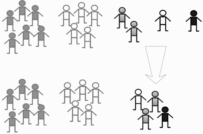
$n$ objects are independently placed into one of $k$ categories, with probability of $p_j$ to category j, and $\sum_{j=1}^k p_j = 1$. Let $X_i$ be the number of objects in category $i$, $X_1 + … + X_n = n$. Then $X = (X_1,…,X_k)$ is said to have Multinomial distribution with parameters $n$ and $\mathbf{p} = (p_1,…,p_k)$, write as $\mathbf{X} \sim Mult_k(n,\mathbf{p})$

Theorem (Multinomial Joint PMF)

If $\mathbf{X}\sim Mult_k(n,\mathbf{p})$, then the joint PMF of $\mathbf{X}$ is

$$P(X_1=n_1,...,X_k=n_k) = \frac{n!}{n_1!n_2!...n_k!}\cdot p_1^{n_1}p_2^{n_2}\dotsb p_k^{n_k}$$

Theorem (Multinomial Marginals)

If $\mathbf{X}\sim Mult_k(n,\mathbf{p})$, then $X_j \sim Bin(n,p_j)$

Theorem (Multinomial Lumping)

If $\mathbf{X}\sim Mult_k(n,\mathbf{p})$, then for distinct $i$ and $j$, $X_i+X_j\sim Bin(n,p_i+p_j)$

$$(X_1+X_2,X_3,...,X_k)\sim Mult_k(n,((p_1+p_2),p_3,...,p_n))$$

Theorem (Multinomial Conditioning)

If $\mathbf{X}\sim Mult_k(n,\mathbf{p})$, then

$$(X_2,...,X_k)|X_1=n_1\sim Mult_k(n-n_1,(p_2^{\prime},...,p_k^{\prime}))$$

where $p_j^{\prime} = p_j/(p_2+\dotsb +p_k)$

Theorem (Covariance in A Multinomial)

Let $X_1,…,X_k\sim Mult_k(n,\mathbf{p})$, where $\mathbf{p} = (p_1,…,p_k)$.

$$Cov(X_i,X_j) = -np_ip_j$$

Definition (Dirichlet Distribution)

Dirichlet distribution is parameterized by a vector $\mathbf{\alpha}$ of positive real numbers. The PDF is:

$$f(p_1,p_2,...,p_k;\alpha_1,\alpha_2,...,\alpha_k)=\frac{\Gamma(\sum_{i=1}^k\alpha_i)}{\prod_{i=1}^k\Gamma(\alpha_i)}\prod_{i=1}^kp_i^{\alpha_i-1}$$

where $p_1 + … + p_k = 1$

Dirichlet-Multinomial Conjugacy

Assume we already have the Multinomial distribution $\mathbf{X}\sim Mult_k(n,\mathbf{p})$. The prior distribution of $\mathbf{p}=(p_1,…,p_k)$ is a Dirichlet distribution, i.e. $\mathbf{p}\sim Dir(\alpha)$. Denote $\mathbf{X} = (X_1,…,X_k)$, then

$$\mathbf{X}|\mathbf{p}\sim Mult_k(n,\mathbf{p})$$

Let $f(\mathbf{p})$ to be the prior distribution of $\mathbf{p}$. The observations of the experiment is $\mathbf{N} = (n_1,…,n_k)$ then

$$\begin{align} f(\mathbf{p}|\mathbf{X}=\mathbf{N}) &= \frac{P(\mathbf{X}=\mathbf{N}|\mathbf{p})f(\mathbf{p})}{P(\mathbf{X}=\mathbf{N})} \\ &= \frac{\frac{n!}{n_1!\dotsb n_k!}p_1^{n_1}\dotsb p_k^{n_k}\cdot \frac{\Gamma(\sum_{i=1}^k \alpha_i)}{\prod_{i=1}^k \Gamma(\alpha_i)}\prod_{i=1}^k p_i^{\alpha_i -1}}{P(\mathbf{X}= \mathbf{N})} \\ &\propto p_1^{n_1+\alpha_1 - 1}\dotsb p_k^{n_k+\alpha_k - 1} \\ &\sim Dir(\mathbf{\alpha} + \mathbf{N}) \end{align}$$

Thus we can see that

$$\text{prior}\ Dir(\mathbf{\alpha}) \rightarrow \text{posterior}\ Dir(\mathbf{\alpha} + \mathbf{N})$$ $$\alpha_i \rightarrow \alpha_i + n_i$$

We can prove that

$$E[p_i|\mathbf{X} = \mathbf{N}] = \frac{\alpha_i + n_i}{\sum_{i=1}^k(\alpha_i + n_i)}$$

---

Bayesian Average

One application for Bayesian Average is in Rating System, usually the customers will rate the movies in 5 star.

This will rose a problem, which One to Choose

• $5$ Average rating movie A by $1$ voter
• $4.9998$ Average rating movie B by $1400010123$ voter (of course this One)

To use the Bayesian estimation to compute the posterior probability for star ratings, we must use a joint distribution, the random variable is a categorical distribution with probability follows:

$$p_1+p_2+p_3+p_4+p_5 = 1$$

Multinomial Distribution

Let $O$ be the event of movie rating, we compute the posterior probability with $N$ observations for five categories with corresponding numbers $K_1,K_2,K_3,K_4,K_5$ as follows:

$$Pr(O|p_1,p_2,p_3,p_4,p_5)\propto p_1^{K_1}p_2^{K_2}p_3^{K_3}p_4^{K_4}p_5^{K_5}$$

where $K_1+…+K_5 = N$

Dirichlet Distribution: Prior

$$Pr(p_1,p_2,p_3,p_4,p_5|O) \propto \prod_{j=1}^5 p_j^{K_j+\alpha_j^0 - 1}$$

After considering the new votes we can update the distribution of the $\mathbf{p}$ by

$$\alpha_j^1 = K_j +\alpha_k^0$$

Expected Average

What we need is the average rating given posterior in the shape of our Dirichlet distribution:

$$E(p_1+2p_2+3p_3+4p_4+5p_5|O) = \sum_{i=1}^5 iE(p_i|O)$$

According to

$$E(p_i|O) = \frac{\alpha_i^1}{\sum_{j=1}^5 \alpha_j^1}$$

We have

$$\sum_{i=1}^5 iE(p_i|O) = \frac{\sum_{i=1}^5 i\alpha_i^0 + \sum_{i=1}^5 i K_i}{\sum_{j=1}^5 \alpha_j^0 +N}$$

Bayesian Average Rating

The final formulation can be express as

$$\text{Bayes Average Rating} = \frac{C\cdot m +\sum(ratings)}{C+N}$$

• N: The number of ratings
• m: a prior for the average of rating scores
• C: a prior for the number of rating scores

---

Gamma Distribution

Definition (Gamma Function)

The Gamma function $\Gamma$ is defined by

$$\Gamma(a) = \int_0^{\infty}x^ae^{-x}\frac{dx}{x}$$

Earlier Beta distribution can represent an unknown probability of success cause its support is $(0,1)$. The Gamma distribution can represent an unknown rate in a Poisson process because its support is $(0,\infty)$

Property of Gamma Function

• $\Gamma(a+1) = a\Gamma(a)$
• $\Gamma(n) = (n-1)!$ if $n$ is a integer

Definition (Gamma Distribution)

An r.v. $Y$ is said to have Gamma distribution with parameters $a>0, \lambda>0$, if its PDF is

$$f(y) = \frac{1}{\Gamma(a)}(\lambda y)^a e^{-\lambda y} \frac{1}{y}, y>0$$

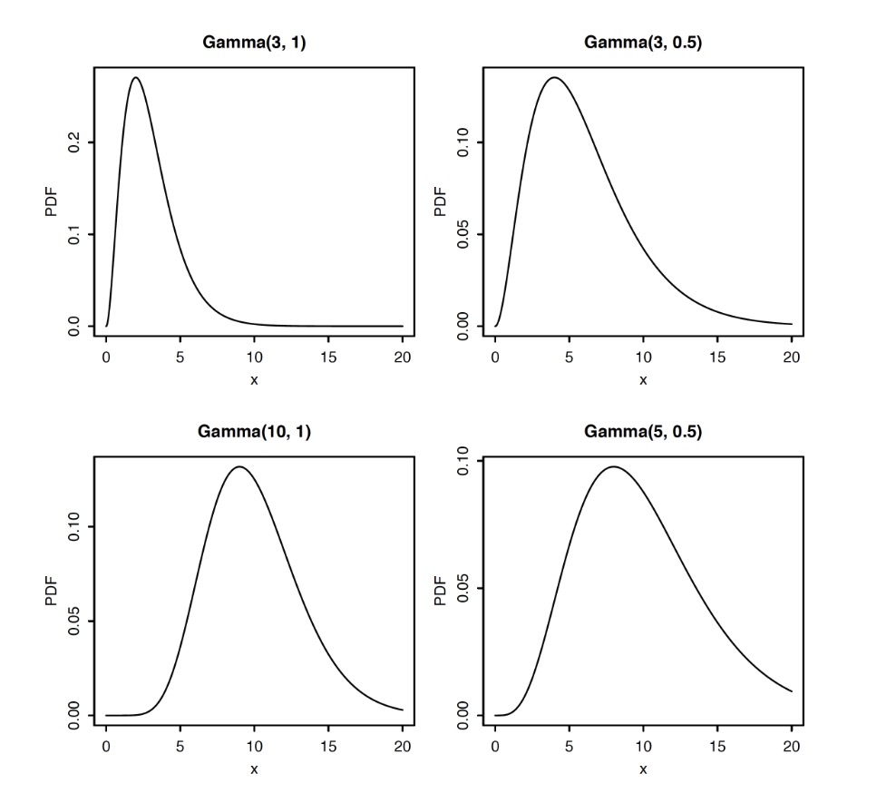
Write $Y\sim Gamma(a,\lambda)$. Gamma distribution is a generalization of exponential distribution when $a=1$

PDF of Gamma distribution

Moments of Gamma Distribution

$$E[X] = \frac{a}{\lambda}, Var(X) = \frac{a}{\lambda^2}$$

Theorem (Gamma: Convolution of Exponential)

Let $X_1,…,X_n$ be i.i.d. $Expo(\lambda)$ , Then

$$X_1+\dotsb +X_n \sim Gamma(n,\lambda)$$

Beta-Gamma Connection

We have independent Gamma r.v.s $X$ and $Y$ with the same rate $\lambda$

• $X+Y$ had Gamma distribution
• $\frac{X}{X+Y}$ has Beta distribution

Binomial & Poisson & Gamma

• The PMF of $Poisson(X=k|\lambda)$ is $P(X=k|\lambda) = \frac{\lambda^ke^{-\lambda}}{k!}$
• The PDF of $X\sim Gamma(a,1)$ is $f_X(x) = \frac{1}{\Gamma(a)}a^{a-1}e^{-x}$. Given $a=k+1$ we have $$P(X=x|a=k+1,1)=\frac{x^{k+1}}{\Gamma(k+1)}e^{-x}= \frac{x^k}{k!}e^{-x}$$
• For a r.v. $X\sim Bin(n,p)$, we have $$P(X\leq k)=\frac{n!}{k!(n-k-1)!}\int_p^1 t^k(1-t)^{n-k-1}dt$$ Let $t=\frac{x}{n}$, then $$P(X\leq k) = \int_{np}^n Bin(X=k|n-1,\frac{x}{n})dx$$ It follows that $$Bin(X\leq k|n,p) = \int_{np}^n Bin(X=k|n-1,\frac{x}{n}dx)$$
• Let $\lambda = np$. We fix $\lambda$, and let $n\rightarrow \infty$, then $$Bin(n,p) \rightarrow Posi(\lambda)$$
• When $\lambda \rightarrow 0$, we have $$1=\mathop{lim}_{\lambda \rightarrow 0} \int_{\lambda}^{\infty} \frac{\lambda^k e^{-x}}{k!}dx = \int_0^{\infty} \frac{x^ke^{-x}}{k!}dx=\int_0^{\infty} Gamma(k+1,1)dx$$
• $1=\int_0^{\infty} \frac{x^ke^{-x}}{k!}dx\Rightarrow k!=\int_0^{\infty}x^k e^{-x}dx$
• Because $Pois(X\leq k|\lambda) = \int_{\lambda}^{\infty}\frac{x^k e^{-x}}{k!} dx$ we have $$Pois(X\leq k|\lambda) + \int_0^{\infty} \frac{x^ke^{-x}}{k!}dx = 1$$

.